excel折线图怎么做？教你Excel做折线图的方法

excel折线图怎么做？在excel表格中我们该如何制作折线呢？在我们使用excel软件制作图表的时候，利用图表能够直观显示表格中的数据，在本文中飞飞系统小编给大家分享介绍下利用excel制作折线的操作方法，利用折线来表现数据分析中经常需要观察数据的走势是非常不错的选择哦！
 

Excel做折线图的方法

这里以wps为例：WPS Office 2016个人免费版 官方免费版

1、打开Excel，选择需要制作的数据，点击“插入”，选择“柱形图”，选择簇状柱状图类型；

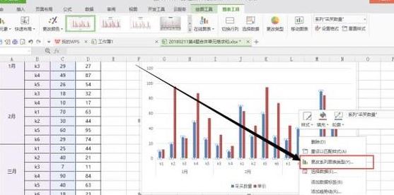
2、将需要设为折线图的数据列选中，鼠标右键点击数据列，选择“更改系列图表类型”；



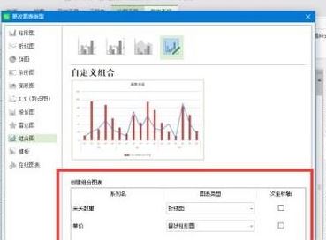
3、在“图表类型”中选择“组合图”，将“采购数量”设置为“折线图”，“单价”设置为“簇状柱形图”，如图：



4、点击“确定”，柱状折线图就制作好



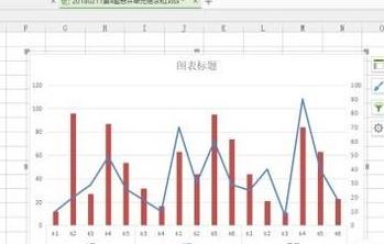
上述便是飞飞系统小编给大家介绍的excel总如何制作折线图的操作方法，希望可以帮到你！